Problem Description and Relevance
The concepts of machine learning and artificial intelligence have been widely used for forecasting the future. One major reason for this recent trend is to use the knowledge of the future to plan out the present perfectly. Some of the major industries who now openly use Machine Learning techniques are claiming that their per capita profit has been drastically increased after the introduction of the new ML techniques. This would explain why the post of Data Scientist and Machine Learning Engineer are being head-hunted by top firms. In the banking sector, customer churn is one of the most important and crucial factors which determine the success of the bank. The problem statement for this project is to predict whether each customer is like to churn within the next month given the details of previous customers who churned from the bank. This is a classic example of a problem in which even though human intelligence is not able to find a correlation, number-crunching machines are able to actively predict the churn of a customer using the data given to the system. One of the most important points that we have to keep in mind is: “Correlation does not guarantee causation”. It simply means that if a feature in the dataset is highly correlated to the output, it does not guarantee that this feature caused the change in output. So, in this project, I will be explaining how to create this geo-demographic model for accurate prediction.
Data Description
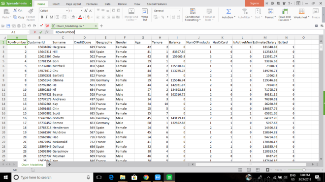
A snapshot of the dataset used for modeling the geo-demographic model is shown above. As you can see, it is a rich dataset in terms of features that we will be using to train the model. A small description of the dataset is given below:
CustomerId- An unique identifier given to each customer of the bank.
Surname- Surname of the customer.
Credit Score- Current credit score for each customer.
Geography- Country where the customer resides in.
Gender- Gender of the customer.
Age- Current age of the customer.
Tenure- Number of loan tenure the customer has at this point in time.
Balance- Current account balance.
NumofProducts- Number of products that customer has subscribed to.
HasCrCard- Boolean variable indicating whether or not the customer has a credit card.
IsActiveMember- Whether the customer is an active member or not.
EstimatedSalary- Estimated Salary of the Customer.
Exited- The target variable; whether the customer exited the bank or not.
A quick glance at this dataset gives us a lot of insight into it. It is quite self-explanatory and we can also easily identify certain features that may be a very big contributor to the prediction of our target variable. For example, the Tenure feature seems to have a very high correlation with the target variable. Some other features like CustomerId are very unlikely to contribute to the target variable at all. What about the rest? It is highly possible for us to underestimate as well as to overestimate the contribution that some of the features may have to the target variable. As a Data Scientist, we will not make any assumptions about such estimations, but rather we will focus on the facts that the data tell us. So, it is highly encouraged to plot the dataset and to the find the mathematical correlation between the various features so that you have a vague idea about the dataset and the dependencies within.
Data Cleaning and Preprocessing
The dataset in hand is generally a very clean one and it doesn’t need to be cleaned anymore. However, some amount of data preprocessing has to be done before the data can be fit to an artificial neural network. As you can see, there are some categorical variables in our dataset, namely, the Gender and Geography. The feature Gender is a binary categorical variable while Geography has multiple categories within. All the categorical variables have to be encoded into numbers before any machine learning algorithm can work on the data. The code snippet below shows the implementation of 2 different but popular methods of encoding the categorical variable: LabelEncoder and OneHotEncoder. The difference between the 2 is very subtle but very important. LabelEncoder simply assigns each category with a random integer. The integers assigned are not in any way comparable to the literal meaning of the categories. OneHotEncoder creates a new column denoting each of the categories possible for the variable. For example, consider the feature Geography which has 3 possible categories Spain, France, and Germany. OneHotEncoder will create a column for each of these possible categories and assign binary values indicating which category the row of data belongs to. On the contrary, LabelEncoder will assign an integer for all of the categories and will not be creating any extra column.
from sklearn.preprocessing import LabelEncoder,OneHotEncoder
labelencoder_X_1=LabelEncoder()
X[:,1]=labelencoder_X_1.fit_transform(X[:,1])
labelencoder_X_2= LabelEncoder()
X[:,2]=labelencoder_X_2.fit_transform(X[:,2])
onehotencoder= OneHotEncoder(categorical_features=[1])
X=onehotencoder.fit_transform(X).toarray()
X=X[:,1:]
The second step in preprocessing will be to apply Feature Scaling. This is a very important step because as you will see further down, ANN works on the values of each feature. If any of these features have values which are overly dominating over the other, the ANN would tend to give more importance to that feature instead of concentrating on the rather important ones. That being said, it is highly advisable to always have a standard scale for all your feature when applying any machine learning algorithm for that matter. There are ML algorithms whose performance is not hindered by the difference in scale of the features, but why take that risk? The below code snippet shows how feature scaling can be done with just a few lines of code in python. Here I am using the StandardScaler class for feature scaling.
from sklearn.preprocessing import StandardScaler
sc=StandardScaler()
X_train=sc.fit_transform(X_train)
X_test= sc.fit_transform(X_test)
Now that we have prepared the data properly, we can get into the fun part: Artificial Neural Networks
Artificial Neural Networks
The Neuron
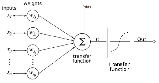
The basic building block of an artificial neural network is the individual neuron. An artificial neural network can be visualized as a graph with individual neurons as the nodes. So, the complete understanding of ANNs cannot be possible without understanding the functioning of individual neurons. Each neuron can have any number of input edges and will have a single output edge. Each of the input edges is associated with a weight which is similar to the edge weight in a weighted graph. Each individual neuron can be thought of performing 2 basic functions:
1) Weighted Sum: Each input is multiplied by the weight of the edge and is summed up in the neuron. In the figure above, this computation is mathematically given by the formula:
S=∑ (X(i)*W(i))+bias
where X(i) is the input at position i and W(i) is the corresponding weight and ∑ is summation over all i.
2) Activation Function: After this sum is computed, the sum is fed into a special function called the activation function. This function can be of various types based on the type of node it appears in. Some of the most popular activation functions are:
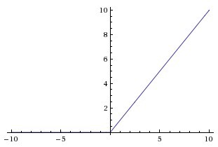
- Rectified Linear Unit (ReLu): One of the most mathematically simple activation functions is the ReLu function. It is highly used in the hidden layers of a neural network as you will soon see.
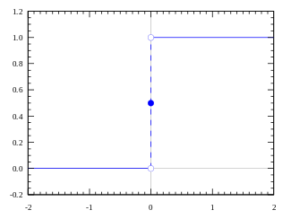
- Threshold Function: It is a simple threshold function whose value is 1 if it is greater than the given threshold or it is 0.
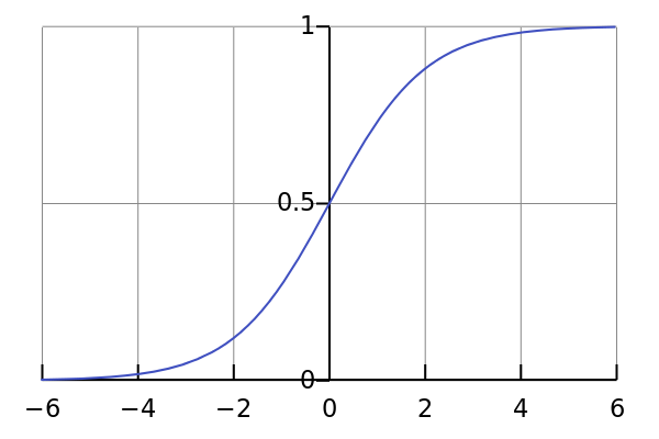
- Sigmoid Function: It is a much more continuous valued function provides the output between 0 and 1. Because of this reason, it is usually used as the activation in the output layer of the ANN.
So, in short, a neuron just does these 2 fundamental functions. A net of neurons forms a neural network. Although a single neuron is not capable of learning, the power that can be derived from a network of neurons is amazing!
The architecture of Neural Networks
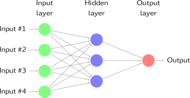
A typical neural network architecture consists of 3 layers: input, hidden and output layers. Each layer can be visualized as an array of individual neurons which is connected to the layer before it. The input layer is the first layer of any neural net. It is a representation of the input data. More accurately, each neuron in the input layer holds the value of each feature of the data on which it is being trained. So, the number of neurons in the input layer will be the number of distinct features that are present in the incoming data. The output layer, as the name suggests, provides the final output of the system. This may be in terms of probability of an event happening, or a real-valued output in case of regression problems. The number of neurons in the output layer can vary from problem to problem. The main feature of a neural network is what is called the hidden layer. This layer of neurons is what gives the neural network the ability to work with more complex problems when compared to other machine learning algorithms.
How does the neural network learn?
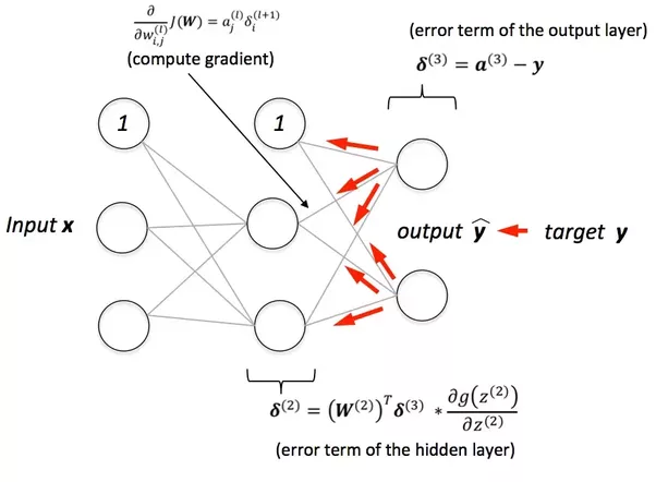
All this sounds interesting, but the golden question is still left unanswered, how does the neural network learn? Without the answer to this questions, all that we know about neural networks is a complete waste. The answer to this all-important question is a single word: backpropagation. Technically, backpropagation is simply a mathematical way to find out the error contributed by each neuron in the network. In simple words, backpropagation tells how responsible a neuron is in the total error in the predictions produced by the system. Lets back up a minute and understand this in an intuitive manner. We know that a neural network is a connection of neurons. Each of the connecting edges has some weight associated with it. The higher the weight of an edge, the more that feature is contributing to the final output. For example, in the problem of predicting bank churn, the feature Credit_Score is one which contributes a lot to the prediction. This statement is equivalent to saying that the weight of the neuron which is connected to the input node representing the credit score will be large. So, basically, the main point to take home is this: the learning of the neural networks comes from getting just the right weights in all the connecting edges between the neurons. And this is exactly what backpropagation helps us to do.
Backpropagation calculates the contribution of each weight in the network towards the final error and either increases or decreases it with the sole purpose of reducing the error. This process of reducing the error is done by a method known as gradient descent. Mathematically, we represent the error produced as a function of the weight and we minimize this error by decreases the gradient at each step. So, in mathematical terms, what backpropagation gives us is the gradient of the function which relates the weight and the error.
Now, another important question to answer is how often do we apply backpropagation. Do we do it after each record/input or do we wait for a batch of records to complete and then apply backpropagation. One of the main motivation for such a question to arise is the complexity of the neural network. A neural network typically has more than one hidden layer and in most cases is fully connected. Although both have their own pros and cons, most machine learning practitioners prefer batch learning because of the time constraints of timing in the training into consideration.
Coding a Neural Network using Keras
Keras is a very helpful wrapper class used for implementing a wide range of neural network architectures. It can be built on both TensorFlow as well as on Theano. This tutorial uses Keras library build on a TensorFlow backend. The first step in using any library is to import it into the current project. In Python, we do it using the import keyword.
import keras
from keras.models import Sequential
from keras.layers import Dense
from keras.layers import Dropout
Sequential is the class for defining a sequential array of neural network layers. In simple words, we use this class to define a neural network where the information flows from right to left or more aptly, from input to output.Sequential model is a linear stack of neural layers. Dense is one of the classes we can use to define a single layer in the neural network. It is one of the core layers of any NN. It is just the regular densely connected neural layer. Dropout is a regularization term used for neural networks. Basically, in each iteration, we deactivate a percentage of the neurons in each layer so as to reduce the learning rate.
classifier= Sequential()
#Adding the input layer adn the first hidden layer with dropout
classifier.add(Dense(output_dim=6,init=’uniform’,activation=’relu’,input_dim=11))
classifier.add(Dropout(p=0.1))
#Adding the second hidden layer
classifier.add(Dense(output_dim=6,init=’uniform’,activation=’relu’))
classifier.add(Dropout(p=0.1))
#Adding the output layer
classifier.add(Dense(output_dim=1,init=’uniform’,activation=’sigmoid’))
This code snippet creates the complete Neural network architecture for the problem defined above. It has an input layer, output layer, and 2 hidden layers. After making the architecture, the next steps would be to compile the network and to train the network on the input data.
#Compiling the ANN
classifier.compile(optimizer=’rmsprop’, loss=’binary_crossentropy’,metrics=[‘accuracy’])
#Fitting the ANN to the training set
classifier.fit(X_train,y_train,batch_size=25,epochs=500)
This might take some while to run, as the NN is training on the input data, making all the complex relationships between the features and the target variable. After training, we can predict on the test set.
y_pred = classifier.predict(X_test)
y_pred= (y_pred> 0.5)
To analyze the performance of the model, we make the confusion matrix and find the mean accuracy, precision, and recall.
from sklearn.metrics import confusion_matrix
cm = confusion_matrix(y_test, y_pred)
Conclusion
In this tutorial, we have successfully implemented an Artificial Neural Network for predicting the bank churn. We have successfully done the data preprocessing, understood what the basic concepts of ANNs are and also implemented the same with python and Keras. I hope you got a little bit more enlightened about ANNs. Until next time, stay curious about AI.